Kurtosis

Statistics: Scientific method · Research methods · Experimental design · Undergraduate statistics courses · Statistical tests · Game theory · Decision theory

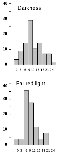
KurtosisChanges — The far red light has no effect on the average speed of the gravitropic reaction in wheat coleoptiles, but it changes kurtosis from platykurtic to leptokurtic (-0.194 → 0.055)

In probability theory and statistics, kurtosis is a measure of the outlier (rare, extreme data) character of the probability distribution of a real-valued random variable. Higher kurtosis means there are infrequent extreme deviations in excess of what is predicted by a normal distribution.

Definition of kurtosis[]

In probability theory and statistics, kurtosis (from Greek: κυρτός, kyrtos or kurtos, meaning "curved, arching") is a measure of the "tailedness" of the probability distribution of a real-valued random variable. In a similar way to the concept of skewness, kurtosis is a descriptor of the shape of a probability distribution and, just as for skewness, there are different ways of quantifying it for a theoretical distribution and corresponding ways of estimating it from a sample from a population. Depending on the particular measure of kurtosis that is used, there are various interpretations of kurtosis, and of how particular measures should be interpreted.

The standard measure of kurtosis, originating with Karl Pearson, is based on a scaled version of the fourth moment of the data or population. This number is related to the tails of the distribution, not its peak;[1] hence, the sometimes-seen characterization as "peakedness" is mistaken. For this measure, higher kurtosis is the result of infrequent extreme deviations (or outliers), as opposed to frequent modestly sized deviations.

The kurtosis of any univariate normal distribution is 3. It is common to compare the kurtosis of a distribution to this value. Distributions with kurtosis less than 3 are said to be platykurtic, although this does not imply the distribution is "flat-topped" as sometimes reported. Rather, it means the distribution produces fewer and less extreme outliers than does the normal distribution. An example of a platykurtic distribution is the uniform distribution, which does not produce outliers. Distributions with kurtosis greater than 3 are said to be leptokurtic. An example of a leptokurtic distribution is the Laplace distribution, which has tails that asymptotically approach zero more slowly than a Gaussian, and therefore produces more outliers than the normal distribution. It is also common practice to use an adjusted version of Pearson's kurtosis, the excess kurtosis, which is the kurtosis minus 3, to provide the comparison to the normal distribution. Some authors use "kurtosis" by itself to refer to the excess kurtosis. For the reason of clarity and generality, however, this article follows the non-excess convention and explicitly indicates where excess kurtosis is meant.

Alternative measures of kurtosis are: the L-kurtosis, which is a scaled version of the fourth L-moment; measures based on four population or sample quantiles.[2] These are analogous to the alternative measures of skewness that are not based on ordinary moments.[2] The fourth standardized moment is defined as μ₄ / σ⁴, where μ₄ is the fourth moment about the mean and σ is the standard deviation. This is sometimes used as the definition of kurtosis in older works, but is not the definition used here.

Kurtosis is more commonly defined as the fourth cumulant divided by the square of the variance of the probability distribution,

\gamma_2 = \frac{\kappa_4}{\kappa_2^2} = \frac{\mu_4}{\sigma^4} - 3, \!

which is known as excess kurtosis. The "minus 3" at the end of this formula is often explained as a correction to make the kurtosis of the normal distribution equal to zero. Another reason can be seen by looking at the formula for the kurtosis of the sum of random variables. Because of the use of the cumulant, if Y is the sum of n independent random variables, all with the same distribution as X, then Kurt[Y] = Kurt[X] / n, while the formula would be more complicated if kurtosis were defined as μ₄ / σ⁴.

More generally, if X₁, ..., X_n are independent random variables all having the same variance, then

\operatorname{Kurt}\left(\sum_{i=1}^n X_i \right) = {1 \over n^2} \sum_{i=1}^n \operatorname{Kurt}(X_i),

whereas this identity would not hold if the definition did not include the subtraction of 3.

Terminology and examples[]

A high kurtosis distribution has a sharper "peak" and fatter "tails", while a low kurtosis distribution has a more rounded peak with wider "shoulders".

Distributions with zero kurtosis are called mesokurtic, or mesokurtotic. The most prominent example of a mesokurtic distribution is the normal distribution family, regardless of the values of its parameters. A few other well-known distributions can be mesokurtic, depending on parameter values: for example the binomial distribution is mesokurtic for $p = 1/2 \pm \sqrt{1/12}$ .

A distribution with positive kurtosis is called leptokurtic, or leptokurtotic. In terms of shape, a leptokurtic distribution has a more acute "peak" around the mean (that is, a higher probability than a normally distributed variable of values near the mean) and "fat tails" (that is, a higher probability than a normally distributed variable of extreme values). Examples of leptokurtic distributions include the Laplace distribution and the logistic distribution.

A distribution with negative kurtosis is called platykurtic, or platykurtotic. In terms of shape, a platykurtic distribution has a smaller "peak" around the mean (that is, a lower probability than a normally distributed variable of values near the mean) and "thin tails" (that is, a lower probability than a normally distributed variable of extreme values). Examples of platykurtic distributions include the continuous or discrete uniform distributions, and the raised cosine distribution. The most platykurtic distribution of all is the Bernoulli distribution with p = ½ (for example the number of times one obtains "heads" when flipping a coin once), for which the kurtosis is -2.

Graphical examples[]

The Pearson type VII family[]

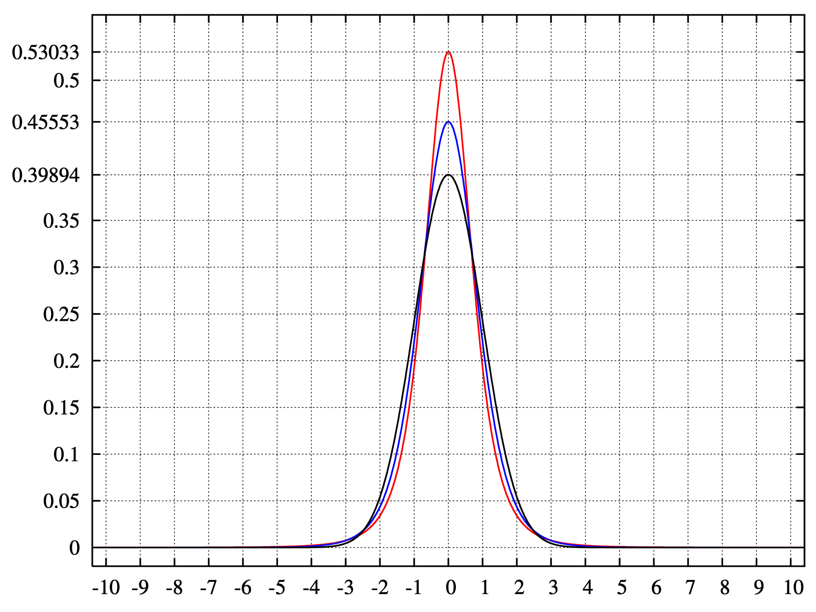
Pearson type VII distribution PDF — pdf for the Pearson type VII distribution with kurtosis of infinity (red); 2 (blue); and 0 (black)

Pearson type VII distribution log-PDF — log-pdf for the Pearson type VII distribution with kurtosis of infinity (red); 2 (blue); 1, 1/2, 1/4, 1/8, and 1/16 (gray); and 0 (black)

We illustrate the effects of kurtosis using a parametric family of distributions whose kurtosis can be adjusted while their lower-order moments and cumulants remain constant. Consider the Pearson type VII family, which is a special case of the Pearson type IV family restricted to symmetric densities. The probability density function is given by

f(x; a, m) = \frac{\Gamma(m)}{a\,\sqrt{\pi}\,\Gamma(m-1/2)} \left[1+\left(\frac{x}{a}\right)^2 \right]^{-m}, \!

where a is a scale parameter and m is a shape parameter.

All densities in this family are symmetric. The kth moment exists provided $m>(k+1)/2$ . For the kurtosis to exist, we require $m>5/2$ . Then the mean and skewness exist and are both identically zero. Setting $a^2 = 2m-3$ makes the variance equal to unity. Then the only free parameter is m, which controls the fourth moment (and cumulant) and hence the kurtosis. One can reparameterize with $m = 5/2 + 3/\gamma_2$ , where $\gamma_2$ is the kurtosis as defined above. This yields a one-parameter leptokurtic family with zero mean, unit variance, zero skewness, and arbitrary positive kurtosis. The reparameterized density is

g(x; \gamma_2) = f(x;\; a=\sqrt{2+6/\gamma_2},\; m=5/2+3/\gamma_2). \!

In the limit as $\gamma_2 \to \infty$ one obtains the density

g(x) = 3 \left(2 + x^2\right)^{-5/2}, \!

which is shown as the red curve in the images on the right.

In the other direction as $\gamma_2 \to 0$ one obtains the standard normal density as the limiting distribution, shown as the black curve.

In the images on the right, the blue curve represents the density $x \mapsto g(x; 2)$ with kurtosis of 2. The top image shows that leptokurtic densities in this family have a higher peak than the mesokurtic normal density. The comparatively fatter tails of the leptokurtic densities are illustrated in the second image, which plots the natural logarithm of the Pearson type VII densities: the black curve is the logarithm of the standard normal density, which is an inverted parabola. One can see that the normal density allocates little probability mass to the regions far from the mean ("has thin tails"), compared with the blue curve of the leptokurtic Pearson type VII density with kurtosis of 2. Between the blue curve and the black are other Pearson type VII densities with γ₂ = 1, 1/2, 1/4, 1/8, and 1/16. The red curve again shows the upper limit of the Pearson type VII family, with $\gamma_2 = \infty$ (which, strictly speaking, means that the fourth moment does not exist). The red curve decreases the slowest as one moves outward from the origin ("has fat tails").

Kurtosis of well-known distributions[]

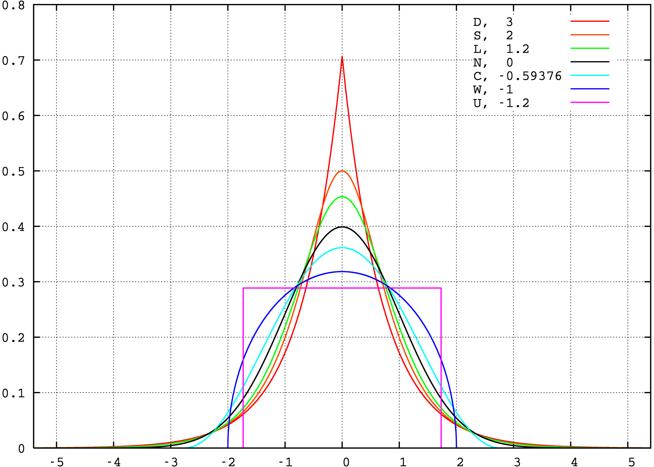
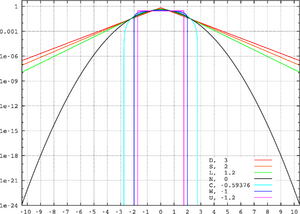
In this example we compare several well-known distributions from different parametric families. All densities considered here are unimodal and symmetric. Each has a mean and skewness of zero. Parameters were chosen to result in a variance of unity in each case. The images on the right show curves for the following seven densities, on a linear scale and logarithmic scale:

D: Laplace distribution, a/k/a double exponential distribution, red curve (two straight lines in the log-scale plot), kurtosis 3 (leptokurtic)
S: hyperbolic secant distribution, orange curve, kurtosis 2 (leptokurtic)
L: logistic distribution, green curve, kurtosis 1.2 (leptokurtic)
N: normal distribution, black curve (inverted parabola in the log-scale plot), kurtosis 0 (mesokurtic)
C: raised cosine distribution, cyan curve, kurtosis −0.593762… (platykurtic)
W: Wigner semicircle distribution, blue curve, kurtosis −1 (platykurtic)
U: uniform distribution, magenta curve (shown for clarity as a rectangle in both images), kurtosis −1.2 (platykurtic)

Note that in this case the platykurtic densities have bounded support, whereas the densities with nonnegative kurtosis are supported on the whole real line. In general there exist platykurtic densities with infinite support, for example exponential power distributions with sufficiently large shape parameter b.

Sample kurtosis[]

For a sample of n values the sample kurtosis is

g_2 = \frac{m_4}{m_{2}^2} -3 = \frac{n\,\sum_{i=1}^n (x_i - \overline{x})^4}{\left(\sum_{i=1}^n (x_i - \overline{x})^2\right)^2} - 3

where m₄ is the fourth sample moment about the mean, m₂ is the second sample moment about the mean (that is, the sample variance), x_i is the i^th value, and $\overline{x}$ is the sample mean.

The formula

D = {1 \over n} \sum_{i=1}^n{ (x_i - \bar{x})^2}

,

E = {1 \over n D^2} \sum_{i=1}^n{ (x_i - \bar{x})^4} - 3

is also used, where n - the sample size, D - the pre-computed variance, x_i - the value of the x'th measurement and $\bar{x}$ - the pre-computed arithmetic mean.

Estimators of population kurtosis[]

Given a sub-set of samples from a population, the sample kurtosis above is a biased estimator of the population kurtosis. The usual estimator of the population kurtosis (used in SAS, SPSS, and Excel but not by MINITAB or BMDP) is G₂, defined as follows:

$G_2 \!\!\!\!$	$= \frac{k_4}{k_{2}^2}\!$
	$= \frac{n^2\,((n+1)\,m_4 - 3\,(n-1)\,m_{2}^2)}{(n-1)\,(n-2)\,(n-3)} \; \frac{(n-1)^2}{n^2\,m_{2}^2}\!$
	$= \frac{n-1}{(n-2)\,(n-3)} \left( (n+1)\,\frac{m_4}{m_{2}^2} - 3\,(n-1) \right)\!$
	$= \frac{n-1}{(n-2) (n-3)} \left( (n+1)\,g_2 + 6 \right)\!$
	$= \frac{(n+1)\,n\,(n-1)}{(n-2)\,(n-3)} \; \frac{\sum_{i=1}^n (x_i - \bar{x})^4}{\left(\sum_{i=1}^n (x_i - \bar{x})^2\right)^2} - 3\,\frac{(n-1)^2}{(n-2)\,(n-3)}\!$
	$= \frac{(n+1)\,n}{(n-1)\,(n-2)\,(n-3)} \; \frac{\sum_{i=1}^n (x_i - \bar{x})^4}{k_{2}^2} - 3\,\frac{(n-1)^2}{(n-2) (n-3)} \!$

where k₄ is the unique symmetric unbiased estimator of the fourth cumulant, k₂ is the unbiased estimator of the population variance, m₄ is the fourth sample moment about the mean, m₂ is the sample variance, x_i is the i^th value, and $\bar{x}$ is the sample mean. Unfortunately, $G_2$ is itself generally biased. For the normal distribution it is unbiased because its expected value is then zero.

References[]

Joanes, D. N. & Gill, C. A. (1998) Comparing measures of sample skewness and kurtosis. Journal of the Royal Statistical Society (Series D): The Statistician 47 (1), 183–189. doi:10.1111/1467-9884.00122

External links[]

Matlab implementation of kurtosis and other statistical measures
Free Online Software (Calculator) computes various types of skewness and kurtosis statistics for any dataset (includes small and large sample tests)..
Kurtosis on the Earliest known uses of some of the words of mathematics
Celebrating 100 years of Kurtosis a history of the topic, with different measures of kurtosis.

This page uses Creative Commons Licensed content from Wikipedia (view authors).