No edit summary |
m (fixing dead links) |
||
| Line 259: | Line 259: | ||
| isbn=0-486-41147-8 |
| isbn=0-486-41147-8 |
||
}}. |
}}. |
||
| − | *John Aldrich, Eigenvalue, eigenfunction, eigenvector, and related terms. In Jeff Miller (Editor), ''[http://members.aol.com/jeff570/e.html Earliest Known Uses of Some of the Words of Mathematics]'', last updated [[7 August]] [[2006]], accessed [[22 August]] [[2006]]. |
+ | *John Aldrich, Eigenvalue, eigenfunction, eigenvector, and related terms. In Jeff Miller (Editor), ''[http://web.archive.org/19990508224238/members.aol.com/jeff570/e.html Earliest Known Uses of Some of the Words of Mathematics]'', last updated [[7 August]] [[2006]], accessed [[22 August]] [[2006]]. |
*{{Citation |
*{{Citation |
||
| last=Strang |
| last=Strang |
||
Revision as of 06:33, 4 November 2013
Assessment |
Biopsychology |
Comparative |
Cognitive |
Developmental |
Language |
Individual differences |
Personality |
Philosophy |
Social |
Methods |
Statistics |
Clinical |
Educational |
Industrial |
Professional items |
World psychology |
Statistics: Scientific method · Research methods · Experimental design · Undergraduate statistics courses · Statistical tests · Game theory · Decision theory

Fig. 1. In this shear mapping of the Mona Lisa, the picture was deformed in such a way that its central vertical axis (red vector) was not modified, but the diagonal vector (blue) has changed direction. Hence the red vector is an eigenvector of the transformation and the blue vector is not. Since the red vector was neither stretched nor compressed, its eigenvalue is 1. All vectors with the same vertical direction - i.e., parallel to this vector - are also eigenvectors, with the same eigenvalue. Together with the zero-vector, they form the eigenspace for this eigenvalue.
In mathematics, a vector may be thought of as an arrow. It has a length, called its magnitude, and it points in some particular direction. A linear transformation may be considered to operate on a vector to change it, usually changing both its magnitude and its direction. An eigenvector of a given linear transformation is a vector which is multiplied by a constant called the eigenvalue during that transformation. The direction of the eigenvector is either unchanged by that transformation (for positive eigenvalues) or reversed (for negative eigenvalues).
For example, an eigenvalue of +2 means that the eigenvector is doubled in length and points in the same direction. An eigenvalue of +1 means that the eigenvector is unchanged, while an eigenvalue of −1 means that the eigenvector is reversed in direction. An eigenspace of a given transformation is the span of the eigenvectors of that transformation with the same eigenvalue, together with the zero vector (which has no direction). An eigenspace is an example of a subspace of a vector space.
In linear algebra, every linear transformation between finite-dimensional vector spaces can be given by a matrix, which is a rectangular array of numbers arranged in rows and columns. Standard methods for finding eigenvalues, eigenvectors, and eigenspaces of a given matrix are discussed below.
These concepts play a major role in several branches of both pure and applied mathematics — appearing prominently in linear algebra, functional analysis, and to a lesser extent in nonlinear mathematics.
Many kinds of mathematical objects can be treated as vectors: functions, harmonic modes, quantum states, and frequencies, for example. In these cases, the concept of direction loses its ordinary meaning, and is given an abstract definition. Even so, if this abstract direction is unchanged by a given linear transformation, the prefix "eigen" is used, as in eigenfunction, eigenmode, eigenstate, and eigenfrequency.
History
Eigenvalues are often introduced in the context of linear algebra or matrix theory. Historically, however, they arose in the study of quadratic forms and differential equations.
Euler had also studied the rotational motion of a rigid body and discovered the importance of the principal axes. As Lagrange realized, the principal axes are the eigenvectors of the inertia matrix.[1] In the early 19th century, Cauchy saw how their work could be used to classify the quadric surfaces, and generalized it to arbitrary dimensions.[2] Cauchy also coined the term racine caractéristique (characteristic root) for what is now called eigenvalue; his term survives in characteristic equation.[3]
Fourier used the work of Laplace and Lagrange to solve the heat equation by separation of variables in his famous 1822 book Théorie analytique de la chaleur.[4] Sturm developed Fourier's ideas further and he brought them to the attention of Cauchy, who combined them with his own ideas and arrived at the fact that symmetric matrices have real eigenvalues.[2] This was extended by Hermite in 1855 to what are now called Hermitian matrices.[3] Around the same time, Brioschi proved that the eigenvalues of orthogonal matrices lie on the unit circle,[2] and Clebsch found the corresponding result for skew-symmetric matrices.[3] Finally, Weierstrass clarified an important aspect in the stability theory started by Laplace by realizing that defective matrices can cause instability.[2]
In the meantime, Liouville studied eigenvalue problems similar to those of Sturm; the discipline that grew out of their work is now called Sturm-Liouville theory.[5] Schwarz studied the first eigenvalue of Laplace's equation on general domains towards the end of the 19th century, while Poincaré studied Poisson's equation a few years later.[6]
At the start of the 20th century, Hilbert studied the eigenvalues of integral operators by viewing the operators as infinite matrices.[7] He was the first to use the German word eigen to denote eigenvalues and eigenvectors in 1904, though he may have been following a related usage by Helmholtz. "Eigen" can be translated as "own", "peculiar to", "characteristic" or "individual"—emphasizing how important eigenvalues are to defining the unique nature of a specific transformation. For some time, the standard term in English was "proper value", but the more distinctive term "eigenvalue" is standard today.[8]
The first numerical algorithm for computing eigenvalues and eigenvectors appeared in 1929, when Von Mises published the power method. One of the most popular methods today, the QR algorithm, was proposed independently by Francis and Kublanovskaya in 1961.[9]
Definitions: the eigenvalue equation
- See also: Eigenplane
Linear transformations of a vector space, such as rotation, reflection, stretching, compression, shear or any combination of these, may be visualized by the effect they produce on vectors. In other words, they are vector functions. More formally, in a vector space L a vector function A is defined if for each vector x of L there corresponds a unique vector y = A(x) of L. For the sake of brevity, the parentheses around the vector on which the transformation is acting are often omitted. A vector function A is linear if it has the following two properties:
- additivity
- homogeneity


where x and y are any two vectors of the vector space L and α is any real number. Such a function is variously called a linear transformation, linear operator, or linear endomorphism on the space L.
|
Given a linear transformation A, a non-zero vector x is defined to be an eigenvector of the transformation if it satisfies the eigenvalue equation for some scalar λ. In this situation, the scalar λ is called an eigenvalue of A corresponding to the eigenvector x. |

The key equation in this definition is the eigenvalue equation, Ax = λx. Most vectors x will not satisfy such an equation. A typical vector x changes direction when acted on by A, so that Ax is not a multiple of x. This means that only certain special vectors x are eigenvectors, and only certain special numbers λ are eigenvalues. Of course, if A is a multiple of the identity matrix, then no vector changes direction, and all non-zero vectors are eigenvectors. But in the usual case, eigenvectors are few and far between. They are the "normal modes" of the system, and they act independently.[10]
The requirement that the eigenvector be non-zero is imposed because the equation A0 = λ0 holds for every A and every λ. Since the equation is always trivially true, it is not an interesting case. In contrast, an eigenvalue can be zero in a nontrivial way. An eigenvalue can be, and usually is, also a complex number. In the definition given above, eigenvectors and eigenvalues do not occur independently. Instead, each eigenvector is associated with a specific eigenvalue. For this reason, an eigenvector x and a corresponding eigenvalue λ are often referred to as an eigenpair. One eigenvalue can be associated with several or even with infinite number of eigenvectors. But conversely, if an eigenvector is given, the associated eigenvalue for this eigenvector is unique. Indeed, from the equality Ax = λx = λ'x and from x ≠ 0 it follows that λ = λ'.[11]
Fig. 2. The eigenvalue equation as a homothety (similarity transformation) on the vector x.
Geometrically (Fig. 2), the eigenvalue equation means that under the transformation A eigenvectors experience only changes in magnitude and sign — the direction of Ax is the same as that of x. This type of linear transformation is defined as homothety (dilatation[12], similarity transformation). The eigenvalue λ is simply the amount of "stretch" or "shrink" to which a vector is subjected when transformed by A. If λ = 1, the vector remains unchanged (unaffected by the transformation). A transformation I under which a vector x remains unchanged, Ix = x, is defined as identity transformation. If λ = –1, the vector flips to the opposite direction (rotates to 180°); this is defined as reflection.
If x is an eigenvector of the linear transformation A with eigenvalue λ, then any vector y = αx is also an eigenvector of A with the same eigenvalue. From the homogeneity of the transformation A it follows that Ay = α(Ax) = α(λx) = λ(αx) = λy. Similarly, using the additivity property of the linear transformation, it can be shown that any linear combination of eigenvectors with eigenvalue λ has the same eigenvalue λ.[13] Therefore, any non-zero vector in the line through x and the zero vector is an eigenvector with the same eigenvalue as x. Together with the zero vector, those eigenvectors form a subspace of the vector space called an eigenspace. The eigenvectors corresponding to different eigenvalues are linearly independent[14] meaning, in particular, that in an n-dimensional space the linear transformation A cannot have more than n eigenvectors with different eigenvalues.[15] The vectors of the eigenspace generate a linear subspace of A which is invariant (unchanged) under this transformation.[16]
If a basis is defined in vector space Ln, all vectors can be expressed in terms of components. Polar vectors can be represented as one-column matrices with n rows where n is the space dimensionality. Linear transformations can be represented with square matrices; to each linear transformation A of Ln corresponds a square matrix of rank n. Conversely, to each square matrix of rank n corresponds a linear transformation of Ln at a given basis. Because of the additivity and homogeneity of the linear trasformation and the eigenvalue equation (which is also a linear transformation — homothety), those vector functions can be expressed in matrix form. Thus, in a the two-dimensional vector space L2 fitted with standard basis, the eigenvector equation for a linear transformation A can be written in the following matrix representation:

where the juxtaposition of matrices means matrix multiplication. This is equivalent to a set of n linear equations, where n is the number of basis vectors in the basis set. In these equations both the eigenvalue λ and the components of x are unknown variables.
The eigenvectors of A as defined above are also called right eigenvectors because they are column vectors that stand on the right side of the matrix A in the eigenvalue equation. If there exists a transposed matrix AT that satifies the eigenvalue equation, that is, if ATx = λx, then λxT = (λx)T = (ATx)T = xTA, or xTA = λxT. The last equation is similar to the eigenvalue equation but instead of the column vector x it contains its transposed vector, the row vector xT, which stands on the left side of the matrix A. The eigenvectors that satisfy the eigenvalue equation xTA = λxT are called left eigenvectors. They are row vectors.[17] In many common applications, only right eigenvectors need to be considered. Hence the unqualified term "eigenvector" can be understood to refer to a right eigenvector. Eigenvalue equations, written in terms of right or left eigenvectors (Ax = λx and xTA = λxT) have the same eigenvalue λ.[18]
An eigenvector is defined to be a principal or dominant eigenvector if it corresponds to the eigenvalue of largest magnitude (for real numbers, largest absolute value). Repeated application of a linear transformation to an arbitrary vector results in a vector proportional (collinear) to the principal eigenvector.[18]
The applicability the eigenvalue equation to general matrix theory extends the use of eigenvectors and eigenvalues to all matrices, and thus greatly extends the scope of use of these mathematical constructs not only to transformations in linear vector spaces but to all fields of science that use matrices: linear equations systems, optimization, vector and tensor calculus, all fields of physics that use matrix quantities, particularly quantum physics, relativity, and electrodynamics, as well as many engineering applications.
Characteristic equation
- Main article: Characteristic equation
- Main article: Characteristic polynomial
The determination of the eigenvalues and eigenvectors is important in virtually all areas of physics and many engineering problems, such as stress calculations, stability analysis, oscillations of vibrating systems, etc. It is equivalent to matrix diagonalization, and is the first step of orthogonalization, finding of invariants, optimization (minimization or maximization), analysis of linear systems, and many other common applications.
The usual method of finding all eigenvectors and eigenvalues of a system is first to get rid of the unknown components of the eigenvectors, then find the eigenvalues, plug those back one by one in the eigenvalue equation in matrix form and solve that as a system of linear equations to find the components of the eigenvectors. From the identity transformation Ix = x, where I is the identity matrix, x in the eigenvalue equation can be replaced by Ix to give:

The identity matrix is needed to keep matrices, vectors, and scalars straight; the equation (A − λ) x = 0 is shorter, but mixed up since it does not differentiate between matrix, scalar, and vector.[19] The expression in the right hand side is transferred to left hand side with a negative sign, leaving 0 on the right hand side:

The eigenvector x is pulled out behind parentheses:

This can be viewed as a linear system of equations in which the coefficient matrix is the expression in the parentheses, the matrix of the unknowns is x, and the right hand side matrix is zero. According to Cramer's rule, this system of equations has non-trivial solutions (not all zeros, or not any number) if and only if its determinant vanishes, so the solutions of the equation are given by:

This equation is defined as the characteristic equation (less often, secular equation) of A, and the left-hand side is defined as the characteristic polynomial. The eigenvector x or its components are not present in the characteristic equation, so at this stage they are dispensed with, and the only unknowns that remain to be calculated are the eigenvalues (the components of matrix A are given, i. e, known beforehand). For a vector space L2, the transformation A is a 2 × 2 square matrix, and the characteristic equation can be written in the following form:

Expansion of the determinant in the left hand side results in a characteristic polynomial which is a monic (its leading coefficient is 1) polynomial of the second degree, and the characteristic equation is the quadratic equation

which has the following solutions (roots):
![{\displaystyle \lambda _{1,2}={\frac {1}{2}}\left[(a_{11}+a_{22})\pm {\sqrt {4a_{12}a_{21}+(a_{11}-a_{22})^{2}}}\right].}](https://services.fandom.com/mathoid-facade/v1/media/math/render/svg/b9bf3f21ce28a3e0b5263479a064479378c61f28)
For real matrices, the coefficients of the characteristic polynomial are all real. The number and type of roots depends on the value of the discriminant, Δ. For cases Δ = 0, Δ > 0, or Δ < 0, respectively, the roots are one real, two real, or two complex. If the roots are complex, they are also complex conjugates of each other. When the number of roots is less than the degree of the characteristic polynomial (the latter is also the rank of the matrix, and the number of dimensions of the vector space) the equation has a multiple root. In the case of a quadratic equation with one root, this root is a double root, or a root with multiplicity 2. A root with a multiplicity of 1 is a simple root. A quadratic equation with two real or complex roots has only simple roots. In general, the algebraic multiplicity of an eigenvalue is defined as the multiplicity of the corresponding root of the characteristic polynomial. The spectrum of a transformation on a finite dimensional vector space is defined as the set of all its eigenvalues. In the infinite-dimensional case, the concept of spectrum is more subtle and depends on the topology of the vector space.
The general formula for the characteristic polynomial of an n-square matrix is

where S0 = 1, S1 = tr(A), the trace of the transformation matrix A, and Sk with k > 1 are the sums of the principal minors of order k.[20] The fact that eigenvalues are roots of an n-order equation shows that a linear transformation of an n-dimensional linear space has at most n different eigenvalues.[21] According to the fundamental theorem of algebra, in a complex linear space, the characteristic polynomial has at least one zero. Consequently, every linear transformation of a complex linear space has at least one eigenvalue. [22][23] For real linear spaces, if the dimension is an odd number, the linear transformation has at least one eigenvalue; if the dimension is an even number, the number of eigenvalues depends on the determinant of the transformation matrix: if the determinant is negative, there exists at least one positive and one negative eigenvalue, if the determinant is positive nothing can be said about existence of eigenvalues.[24] The complexity of the problem for finding roots/eigenvalues of the characteristic polynomial increases rapidly with increasing the degree of the polynomial (the dimension of the vector space), n. Thus, for n = 3, eigenvalues are roots of the cubic equation, for n = 4 — roots of the quartic equation. For n > 4 there are no exact solutions and one has to resort to root-finding algorithms, such as Newton's method (Horner's method) to find numerical approximations of eigenvalues. For large symmetric sparse matrices, Lanczos algorithm is used to compute eigenvalues and eigenvectors.
In order to find the eigenvectors, the eigenvalues thus found as roots of the characteristic equations are plugged back, one at a time, in the eigenvalue equation written in a matrix form (illustrated for the simplest case of a two-dimensional vector space L2):

where λ is one of the eigenvalues found as a root of the characteristic equation. This matrix equation is equivalent to a system of two linear equations:

The equations are solved for x and y by the usual algebraic or matrix methods. Often, it is possible to divide both sides of the equations to one or more of the coefficients which makes some of the coefficients in front of the unknowns equal to 1. This is called normalization of the vectors, and corresponds to choosing one of the eigenvectors (the normalized eigenvector) as a representative of all vectors in the eigenspace corresponding to the respective eigenvalue. The x and y thus found are the components of the eigenvector in the coordinate system used (most often Cartesian, or polar).
Using the Cayley-Hamilton theorem which states that every square matrix satisfies its own characteristic equation, it can be shown that (most generally, in the complex space) there exists at least one non-zero vector that satisfies the eigenvalue equation for that matrix.[25] As it was said in the Definitions section, to each eigenvalue correspond an infinite number of colinear (linearly dependent) eigenvectors that form the eigenspace for this eigenvalue. On the other hand, the dimension of the eigenspace is equal to the number of the linearly independent eigenvectors that it contains. The geometric multiplicity of an eigenvalue is defined as the dimension of the associated eigenspace. A multiple eigenvalue may give rise to a single eigenvector so that its algebraic multiplicity may be different than the geometric multiplicity.[26] However, as already stated, different eigenvalues are paired with linearly independent eigenvectors.[14] From the aforementioned, it follows that the geometric multiplicity cannot be greater than the algebraic multiplicity.[27]
For instance, an eigenvector of a rotation in three dimensions is a vector located within the axis about which the rotation is performed. The corresponding eigenvalue is 1 and the corresponding eigenspace contains all the vectors along the axis. As this is a one-dimensional space, its geometric multiplicity is one. This is the only eigenvalue of the spectrum (of this rotation) that is a real number.
Examples
The examples that follow are for the simplest case of two-dimensional vector space L2 but they can easily be applied in the same manner to spaces of higher dimensions.
Homothety, identity, point reflection, and null transformation
Fig. 3. When a surface is stretching equally in homothety, any one of the radial vectors can be the eigenvector.
As a one-dimensional vector space L1, consider a rubber string tied to unmoving support in one end, such as that on a child's sling. Pulling the string away from the point of attachment stretches it and elongates it by some scaling factor λ which is a real number. Each vector on the string is stretched equally, with the same scaling factor λ, and although elongated it preserves its original direction. This type of transformation is called homothety (similarity transformation). For a two-dimensional vector space L2, consider a rubber sheet stretched equally in all directions such as a small area of the surface of an inflating balloon (Fig. 3). All vectors originating at a fixed point on the balloon surface are stretched equally with the same scaling factor λ. The homothety transformation in two-dimensions is described by a 2 × 2 square matrix, acting on an arbitrary vector in the plane of the stretching/shrinking surface. After doing the matrix multiplication, one obtains:

which, expressed in words, means that the transformation is equivalent to multiplying the length of the vector by λ while preserving its original direction. The equation thus obtained is exactly the eigenvalue equation. Since the vector taken was arbitrary, in homothety any vector in the vector space undergoes the eigenvalue equation, i. e. any vector lying on the balloon surface can be an eigenvector. Whether the transformation is stretching (elongation, extension, inflation), or shrinking (compression, deflation) depends on the scaling factor: if λ > 1, it is stretching, if λ < 1, it is shrinking.
Several other transformations can be considered special types of homothety with some fixed, constant value of λ: in identity which leaves vectors unchanged, λ = 1; in reflection about a point which preserves length and direction of vectors but changes their orientation to the opposite one, λ = −1; and in null transformation which transforms each vector to the zero vector, λ = 0. The null transformation does not give rise to an eigenvector since the zero vector cannot be an eigenvector but it has eigenspace since eigenspace contains also the zero vector by definition.
Unequal scaling
For a slightly more complicated example, consider a sheet that is stretched uneqally in two perpendicular directions along the coordinate axes, or, similarly, stretched in one direction, and shrunk in the other direction. In this case, there are two different scaling factors: k1 for the scaling in direction x, and k2 for the scaling in direction y. The transformation matrix is , and the characteristic equation is λ2 − λ (k1 + k2) + k1k2 = 0. The eigenvalues, obtained as roots of this equation are λ1 = k1, and λ2 = k2 which means, as expected, that the two eigenvalues are the scaling factors in the two directions. Plugging k1 back in the eigenvalue equation gives one of the eigenvectors:


Dividing the last equation by k2 − k1, one obtains y = 0 which represents the x axis. A vector with lenght 1 taken along this axis represents the normalized eigenvector corresponding to the eigenvalue λ1. The eigenvector corresponding to λ2 which is a unit vector along the y axis is found in a similar way. In this case, both eigenvalues are simple (with algebraic and geometric multiplicities equal to 1). Depending on the values of λ1 and λ2, there are several notable special cases. In particular, if λ1 > 1, and λ2 = 1, the transformation is a stretch in the direction of axis x. If λ2 = 0, and λ1 = 1, the transformation is a projection of the surface L2 on the axis x because all vectors in the direction of y become zero vectors.
Let the rubber sheet is stretched along the x axis (k1 > 1) and simultaneously shrunk along the y axis (k2 < 1). Then λ1 = k1 will be the principal eigenvalue. Repeatedly applying this transformation of stretching/shrinking many times to the rubber sheet will turn the latter more and more similar to a rubber string. Any vector on the surface of the rubber sheet will be oriented closer and closer to the direction of the x axis (the direction of stretching), that is, it will become collinear with the principal eigenvector.
Mona Lisa
For the example shown on the right, the matrix that would produce a shear transformation similar to this would be

The set of eigenvectors for is defined as those vectors which, when multiplied by , result in a simple scaling of . Thus,


If we restrict ourselves to real eigenvalues, the only effect of the matrix on the eigenvectors will be to change their length, and possibly reverse their direction. So multiplying the right hand side by the Identity matrix I, we have

and therefore

In order for this equation to have non-trivial solutions, we require the determinant , which is called the characteristic polynomial of the matrix A, to be zero. In our example we can calculate the determinant as


and now we have obtained the characteristic polynomial of the matrix A. There is in this case only one distinct solution of the equation , . This is the eigenvalue of the matrix A. As in the study of roots of polynomials, it is convenient to say that this eigenvalue has multiplicity 2.


Having found an eigenvalue , we can solve for the space of eigenvectors by finding the nullspace of . In other words by solving for vectors which are solutions of


Substituting our obtained eigenvalue ,

Solving this new matrix equation, we find that vectors in the nullspace have the form

where c is an arbitrary constant. All vectors of this form, i.e. pointing straight up or down, are eigenvectors of the matrix A. The effect of applying the matrix A to these vectors is equivalent to multiplying them by their corresponding eigenvalue, in this case 1.
In general, 2-by-2 matrices will have two distinct eigenvalues, and thus two distinct eigenvectors. Whereas most vectors will have both their lengths and directions changed by the matrix, eigenvectors will only have their lengths changed, and will not change their direction, except perhaps to flip through the origin in the case when the eigenvalue is a negative number. Also, it is usually the case that the eigenvalue will be something other than 1, and so eigenvectors will be stretched, squashed and/or flipped through the origin by the matrix.
Other examples
As the Earth rotates, every arrow pointing outward from the center of the Earth also rotates, except those arrows which are parallel to the axis of rotation. Consider the transformation of the Earth after one hour of rotation: An arrow from the center of the Earth to the Geographic South Pole would be an eigenvector of this transformation, but an arrow from the center of the Earth to anywhere on the equator would not be an eigenvector. Since the arrow pointing at the pole is not stretched by the rotation of the Earth, its eigenvalue is 1.
Fig. 2. A standing wave in a rope fixed at its boundaries is an example of an eigenvector, or more precisely, an eigenfunction of the transformation giving the acceleration. As time passes, the standing wave is scaled by a sinusoidal oscillation whose frequency is determined by the eigenvalue, but its overall shape is not modified.
However, three-dimensional geometric space is not the only vector space. For example, consider a stressed rope fixed at both ends, like the vibrating strings of a string instrument (Fig. 2). The distances of atoms of the vibrating rope from their positions when the rope is at rest can be seen as the components of a vector in a space with as many dimensions as there are atoms in the rope.
Assume the rope is a continuous medium. If one considers the equation for the acceleration at every point of the rope, its eigenvectors, or eigenfunctions, are the standing waves. The standing waves correspond to particular oscillations of the rope such that the acceleration of the rope is simply its shape scaled by a factor—this factor, the eigenvalue, turns out to be where is the angular frequency of the oscillation. Each component of the vector associated with the rope is multiplied by a time-dependent factor . If damping is considered, the amplitude of this oscillation decreases until the rope stops oscillating, corresponding to a complex ω. One can then associate a lifetime with the imaginary part of ω, and relate the concept of an eigenvector to the concept of resonance. Without damping, the fact that the acceleration operator (assuming a uniform density) is Hermitian leads to several important properties, such as that the standing wave patterns are orthogonal functions.


Eigenfunctions
However, it is sometimes unnatural or even impossible to write down the eigenvalue equation in a matrix form. This occurs for instance when the vector space is infinite dimensional, for example, in the case of the rope above. Depending on the nature of the transformation T and the space to which it applies, it can be advantageous to represent the eigenvalue equation as a set of differential equations. If T is a differential operator, the eigenvectors are commonly called eigenfunctions of the differential operator representing T. For example, differentiation itself is a linear transformation since

(f(t) and g(t) are differentiable functions, and a and b are constants).
Consider differentiation with respect to . Its eigenfunctions h(t) obey the eigenvalue equation:

- ,

where λ is the eigenvalue associated with the function. Such a function of time is constant if , grows proportionally to itself if is positive, and decays proportionally to itself if is negative. For example, an idealized population of rabbits breeds faster the more rabbits there are, and thus satisfies the equation with a positive lambda.

The solution to the eigenvalue equation is , the exponential function; thus that function is an eigenfunction of the differential operator d/dt with the eigenvalue λ. If λ is negative, we call the evolution of g an exponential decay; if it is positive, an exponential growth. The value of λ can be any complex number. The spectrum of d/dt is therefore the whole complex plane. In this example the vector space in which the operator d/dt acts is the space of the differentiable functions of one variable. This space has an infinite dimension (because it is not possible to express every differentiable function as a linear combination of a finite number of basis functions). However, the eigenspace associated with any given eigenvalue λ is one dimensional. It is the set of all functions , where A is an arbitrary constant, the initial population at t=0.


Spectral theorem
- For more details on this topic, see spectral theorem.
In its simplest version, the spectral theorem states that, under certain conditions, a linear transformation of a vector can be expressed as a linear combination of the eigenvectors, in which the coefficient of each eigenvector is equal to the corresponding eigenvalue times the scalar product (or dot product) of the eigenvector with the vector . Mathematically, it can be written as:


where and stand for the eigenvectors and eigenvalues of . The theorem is valid for all self-adjoint linear transformations (linear transformations given by real symmetric matrices and Hermitian matrices), and for the more general class of (complex) normal matrices.


If one defines the nth power of a transformation as the result of applying it n times in succession, one can also define polynomials of transformations. A more general version of the theorem is that any polynomial P of is given by

The theorem can be extended to other functions of transformations, such as analytic functions, the most general case being Borel functions.
Eigendecomposition
- Main article: Eigendecomposition (matrix)
The spectral theorem for matrices can be stated as follows. Let be a square () matrix. Let be an eigenvector basis, i.e. an indexed set of k linearly independent eigenvectors, where k is the dimension of the space spanned by the eigenvectors of . If k=n, then can be written


where is the square () matrix whose ith column is the basis eigenvector of and is the diagonal matrix whose diagonal elements are the corresponding eigenvalues, i.e. .


Infinite-dimensional spaces
If the vector space is an infinite dimensional Banach space, the notion of eigenvalues can be generalized to the concept of spectrum. The spectrum is the set of scalars λ for which is not defined; that is, such that has no bounded inverse.


Clearly if λ is an eigenvalue of T, λ is in the spectrum of T. In general, the converse is not true. There are operators on Hilbert or Banach spaces which have no eigenvectors at all. This can be seen in the following example. The bilateral shift on the Hilbert space (the space of all sequences of scalars such that converges) has no eigenvalue but has spectral values.


In infinite-dimensional spaces, the spectrum of a bounded operator is always nonempty. This is also true for an unbounded self adjoint operator. Via its spectral measures, the spectrum of any self adjoint operator, bounded or otherwise, can be decomposed into absolutely continuous, pure point, and singular parts. (See Decomposition of spectrum.)
Exponential functions are eigenfunctions of the derivative operator (the derivative of exponential functions are proportional to themself). Exponential growth and decay therefore provide examples of continuous spectra, as does the vibrating string example illustrated above. The hydrogen atom is an example where both types of spectra appear. The eigenfunctions of the hydrogen atom Hamiltonian are called eigenstates and are grouped into two categories. The bound states of the hydrogen atom correspond to the discrete part of the spectrum (they have a discrete set of eigenvalues which can be computed by Rydberg formula) while the ionization processes are described by the continuous part (the energy of the collision/ionization is not quantified).
Applications
Schrödinger equation

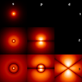
Fig. 4. The wavefunctions associated with the bound states of an electron in a hydrogen atom can be seen as the eigenvectors of the hydrogen atom Hamiltonian as well as of the angular momentum operator. They are associated with eigenvalues interpreted as their energies (increasing downward: n=1,2,3,...) and angular momentum (increasing across: s, p, d,...). The illustration shows the square of the absolute value of the wavefunctions. Brighter areas correspond to higher probability density for a position measurement. The center of each figure is the atomic nucleus, a proton.
An example of an eigenvalue equation where the transformation is represented in terms of a differential operator is the time-independent Schrödinger equation in quantum mechanics:

where H, the Hamiltonian, is a second-order differential operator and , the wavefunction, is one of its eigenfunctions corresponding to the eigenvalue E, interpreted as its energy.

However, in the case where one is interested only in the bound state solutions of the Schrödinger equation, one looks for within the space of square integrable functions. Since this space is a Hilbert space with a well-defined scalar product, one can introduce a basis set in which and H can be represented as a one-dimensional array and a matrix respectively. This allows one to represent the Schrödinger equation in a matrix form. (Fig. 4 presents the lowest eigenfunctions of the Hydrogen atom Hamiltonian.)
The Dirac notation is often used in this context. A vector, which represents a state of the system, in the Hilbert space of square integrable functions is represented by . In this notation, the Schrödinger equation is:


where is an eigenstate of H. It is a self adjoint operator, the infinite dimensional analog of Hermitian matrices (see Observable). As in the matrix case, in the equation above is understood to be the vector obtained by application of the transformation H to .

Molecular orbitals
In quantum mechanics, and in particular in atomic and molecular physics, within the Hartree-Fock theory, the atomic and molecular orbitals can be defined by the eigenvectors of the Fock operator. The corresponding eigenvalues are interpreted as ionization potentials via Koopmans' theorem. In this case, the term eigenvector is used in a somewhat more general meaning, since the Fock operator is explicitly dependent on the orbitals and their eigenvalues. If one wants to underline this aspect one speaks of implicit eigenvalue equation. Such equations are usually solved by an iteration procedure, called in this case self-consistent field method. In quantum chemistry, one often represents the Hartree-Fock equation in a non-orthogonal basis set. This particular representation is a generalized eigenvalue problem called Roothaan equations.
Geology and Glaciology: (Orientation Tensor)
In geology, especially in the study of glacial till, eigenvectors and eigenvalues are used as a method by which a mass of information of a clast fabric's constituents' orientation and dip can be summarized in a 3-D space by six numbers. In the field, a geologist may collect such data for hundreds or thousands of clasts in a soil sample, which can only be compared graphically such as in a Tri-Plot (Sneed and Folk) diagram [28], [29], or as a Stereonet on a Wulff Net [30]. The output for the orientation tensor is in the three orthogonal (perpendicular) axes of space. Eigenvectors output from programs such as Stereo32 [31] are in the order E1 > E2 > E3, with E1 being the primary orientation of clast orientation/dip, E2 being the secondary and E3 being the tertiary, in terms of strength. The clast orientation is defined as the Eigenvector, on a compass rose of 360°. Dip is measured as the Eigenvalue, the modulus of the tensor: this is valued from 0° (no dip) to 90° (vertical). Various values of E1, E2 and E3 mean different things, as can be seen in the book 'A Practical Guide to the Study of Glacial Sediments' by Benn & Evans, 2004 [32].
Factor analysis
In factor analysis, the eigenvectors of a covariance matrix or correlation matrix correspond to factors, and eigenvalues to the variance explained by these factors. Factor analysis is a statistical technique used in the social sciences and in marketing, product management, operations research, and other applied sciences that deal with large quantities of data. The objective is to explain most of the covariability among a number of observable random variables in terms of a smaller number of unobservable latent variables called factors. The observable random variables are modeled as linear combinations of the factors, plus unique variance terms. Eigenvalues are used in analysis used by Q-methodology software; factors with eigenvalues greater than 1.00 are considered significant, explaining an important amount of the variability in the data, while eigenvalues less than 1.00 are considered too weak, not explaining a significant portion of the data variability.

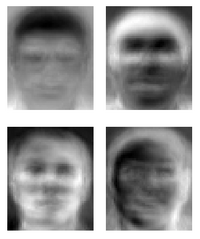
Fig. 5. Eigenfaces as examples of eigenvectors
Eigenfaces
In image processing, processed images of faces can be seen as vectors whose components are the brightnesses of each pixel. The dimension of this vector space is the number of pixels. The eigenvectors of the covariance matrix associated to a large set of normalized pictures of faces are called eigenfaces. They are very useful for expressing any face image as a linear combination of some of them. In the facial recognition branch of biometrics, eigenfaces provide a means of applying data compression to faces for identification purposes. Research related to eigen vision systems determining hand gestures has also been made. More on determining sign language letters using eigen systems can be found here: http://www.geigel.com/signlanguage/index.php
Similar to this concept, eigenvoices concept is also developed which represents the general direction of variability in human pronunciations of a particular utterance, such as a word in a language. Based on a linear combination of such eigenvoices, a new voice pronunciation of the word can be constructed. These concepts have been found useful in automatic speech recognition systems, for speaker adaptation.
Tensor of inertia
In mechanics, the eigenvectors of the inertia tensor define the principal axes of a rigid body. The tensor of inertia is a key quantity required in order to determine the rotation of a rigid body around its center of mass.
Stress tensor
In solid mechanics, the stress tensor is symmetric and so can be decomposed into a diagonal tensor with the eigenvalues on the diagonal and eigenvectors as a basis. Because it is diagonal, in this orientation, the stress tensor has no shear components; the components it does have are the principal components.
Eigenvalues of a graph
In spectral graph theory, an eigenvalue of a graph is defined as an eigenvalue of the graph's adjacency matrix A, or (increasingly) of the graph's Laplacian matrix, which is either T−A or I−T 1/2AT −1/2, where T is a diagonal matrix holding the degree of each vertex, and in T −1/2, 0 is substituted for 0−1/2. The kth principal eigenvector of a graph is defined as either the eigenvector corresponding to the kth largest eigenvalue of A, or the eigenvector corresponding to the kth smallest eigenvalue of the Laplacian. The first principal eigenvector of the graph is also referred to merely as the principal eigenvector.
The principal eigenvector is used to measure the centrality of its vertices. An example is Google's PageRank algorithm. The principal eigenvector of a modified adjacency matrix of the World Wide Web graph gives the page ranks as its components. This vector corresponds to the stationary distribution of the Markov chain represented by the row-normalized adjacency matrix; however, the adjacency matrix must first be modified to ensure a stationary distribution exists. The second principal eigenvector can be used to partition the graph into clusters, via spectral clustering.
See also
- Nonlinear eigenproblem
- Quadratic eigenvalue problem
Notes
- ↑ See Hawkins (1975), §2.
- ↑ 2.0 2.1 2.2 2.3 See Hawkins (1975), §3.
- ↑ 3.0 3.1 3.2 See Kline 1972, pp. 807-808
- ↑ See Kline 1972, p. 673
- ↑ See Kline 1972, pp. 715-716
- ↑ See Kline 1972, pp. 706-707
- ↑ See Kline 1972, p. 1063
- ↑ See Aldrich (2006).
- ↑ See Golub & van Loan 1996, §7.3; Meyer 2000, §7.3
- ↑ See Strang 2006, p. 249
- ↑ See Sharipov 1996, p. 66
- ↑ See Bowen & Wang 1980, p. 148
- ↑ For a proof of this lemma, see Shilov 1969, p. 131, and Lemma for the eigenspace
- ↑ 14.0 14.1 For a proof of this lemma, see Shilov 1969, p. 130, Hefferon 2001, p. 364, and Lemma for linear independence of eigenvectors
- ↑ See Shilov 1969, p. 131
- ↑ For proof, see Sharipov 1996, Theorem 4.4 on p. 68
- ↑ See Shores 2007, p. 252
- ↑ 18.0 18.1 For a proof of this theorem, see Weisstein, Eric W. Eigenvector From MathWorld − A Wolfram Web Resource
- ↑ See Strang 2006, footnote to p. 245
- ↑ For details and proof, see Meyer 2000, p. 494-495
- ↑ See Greub 1975, p. 118
- ↑ See Greub 1975, p. 119
- ↑ For proof, see Gelfand 1971, p. 115
- ↑ For proof, see Greub 1975, p. 119
- ↑ For details and proof, see Kuttler 2007, p. 151
- ↑ See Shilov 1969, p. 134
- ↑ See Shilov 1969, p. 135 and Problem 11 to Chapter 5
- ↑ Graham, D., and Midgley, N., 2000. Earth Surface Processes and Landforms (25) pp 1473-1477
- ↑ Sneed ED, Folk RL. 1958. Pebbles in the lower Colorado River, Texas, a study of particle morphogenesis. Journal of Geology 66(2): 114–150
- ↑ GIS-stereoplot: an interactive stereonet plotting module for ArcView 3.0 geographic information system
- ↑ Stereo32
- ↑ Benn, D., Evans, D., 2004. A Practical Guide to the study of Glacial Sediments. London: Arnold. pp 103-107
References
- Korn, Granino A.; Korn, Theresa M. (2000), Mathematical Handbook for Scientists and Engineers: Definitions, Theorems, and Formulas for Reference and Review, 1152 p., Dover Publications, 2 Revised edition, ISBN 0-486-41147-8.
- John Aldrich, Eigenvalue, eigenfunction, eigenvector, and related terms. In Jeff Miller (Editor), Earliest Known Uses of Some of the Words of Mathematics, last updated 7 August 2006, accessed 22 August 2006.
- Strang, Gilbert (1993), Introduction to linear algebra, Wellesley-Cambridge Press, Wellesley, MA, ISBN 0-961-40885-5.
- Strang, Gilbert (2006), Linear algebra and its applications, Thomson, Brooks/Cole, Belmont, CA, ISBN 0-030-10567-6.
- Bowen, Ray M.; Wang, Chao-Cheng (1980), Linear and multilinear algebra, Plenum Press, New York, NY, ISBN 0-306-37508-7.
- Claude Cohen-Tannoudji, Quantum Mechanics, Wiley (1977). ISBN 0-471-16432-1. (Chapter II. The mathematical tools of quantum mechanics.)
- John B. Fraleigh and Raymond A. Beauregard, Linear Algebra (3rd edition), Addison-Wesley Publishing Company (1995). ISBN 0-201-83999-7 (international edition).
- Golub, Gene H.; van Loan, Charles F. (1996), Matrix computations (3rd Edition), Johns Hopkins University Press, Baltimore, MD, ISBN 978-0-8018-5414-9.
- T. Hawkins, Cauchy and the spectral theory of matrices, Historia Mathematica, vol. 2, pp. 1–29, 1975.
- Roger A. Horn and Charles R. Johnson, Matrix Analysis, Cambridge University Press, 1985. ISBN 0-521-30586-1 (hardback), ISBN 0-521-38632-2 (paperback).
- Kline, Morris (1972), Mathematical thought from ancient to modern times, Oxford University Press, ISBN 0-195-01496-0.
- Meyer, Carl D. (2000), Matrix analysis and applied linear algebra, Society for Industrial and Applied Mathematics (SIAM), Philadelphia, ISBN 978-0-89871-454-8.
- Brown, Maureen, "Illuminating Patterns of Perception: An Overview of Q Methodology" October 2004
- Gene H. Golub and Henk A. van der Vorst, "Eigenvalue computation in the 20th century," Journal of Computational and Applied Mathematics 123, 35-65 (2000).
- Max A. Akivis and Vladislav V. Goldberg, Tensor calculus (in Russian), Science Publishers, Moscow, 1969.
- Gelfand, I. M. (1971), Lecture notes in linear algebra, Russian: Science Publishers, Moscow
- Pavel S. Alexandrov, Lecture notes in analytical geometry (in Russian), Science Publishers, Moscow, 1968.
- Carter, Tamara A., Richard A. Tapia, and Anne Papaconstantinou, Linear Algebra: An Introduction to Linear Algebra for Pre-Calculus Students, Rice University, Online Edition, Retrieved on 2008-02-19.
- Steven Roman, Advanced linear algebra 3rd Edition, Springer Science + Business Media, LLC, New York, NY, 2008. ISBN 978-0-387-72828-5
- Shilov, G. E. (1969), Finite-dimensional (linear) vector spaces, Russian: State Technical Publishing House, 3rd Edition, Moscow.
- Hefferon, Jim (2001), Linear Algebra, Online book, St Michael's College, Colchester, Vermont, USA, http://joshua.smcvt.edu/linearalgebra/.
- Kuttler, Kenneth (2007), An introduction to linear algebra, Online e-book in PDF format, Brigham Young University, http://www.math.byu.edu/~klkuttle/Linearalgebra.pdf.
- James W. Demmel, Applied Numerical Linear Algebra, SIAM, 1997, ISBN 0-89871-389-7.
- Robert A. Beezer, A First Course In Linear Algebra, Free online book under GNU licence, University of Puget Sound, 2006
- Lancaster, P. Matrix Theory (in Russian), Science Publishers, Moscow, 1973, 280 p.
- Paul R. Halmos, Finite-Dimensional Vector Spaces, 8th Edition, Springer-Verlag, New York, 1987, 212 p., ISBN 0387900934
- Pigolkina, T. S. and Shulman, V. S., Eigenvalue (in Russian), In:Vinogradov, I. M. (Ed.), Mathematical Encyclopedia, Vol. 5, Soviet Encyclopedia, Moscow, 1977.
- Pigolkina, T. S. and Shulman, V. S., Eigenvector (in Russian), In:Vinogradov, I. M. (Ed.), Mathematical Encyclopedia, Vol. 5, Soviet Encyclopedia, Moscow, 1977.
- Greub, Werner H. (1975), Linear Algebra (4th Edition), Springer-Verlag, New York, NY, ISBN 0-387-90110-8.
- Larson, Ron and Bruce H. Edwards, Elementary Linear Algebra, 5th Edition, Houghton Mifflin Company, 2003, ISBN 0618335676.
- Curtis, Charles W., Linear Algebra: An Introductory Approach, 347 p., Springer; 4th ed. 1984. Corr. 7th printing edition (August 19, 1999), ISBN 0387909923.
- Shores, Thomas S. (2007), Applied linear algebra and matrix analysis, Springer Science+Business Media, LLC, ISBN 0-387-33194-8.
- Sharipov, Ruslan A. (1996), Course of Linear Algebra and Multidimensional Geometry: the textbook, Online e-book in PDF format, Bashkir State University, Ufa, arXiv:math/0405323v1, ISBN 5-7477-0099-5, http://www.geocities.com/r-sharipov.
External links
- MIT Video Lecture on Eigenvalues and Eigenvectors at Google Video, from MIT OpenCourseWare
- ARPACK is a collection of FORTRAN subroutines for solving large scale (sparse) eigenproblems.
- IRBLEIGS, has MATLAB code with similar capabilities to ARPACK. (See this paper for a comparison between IRBLEIGS and ARPACK.)
- LAPACK is a collection of FORTRAN subroutines for solving dense linear algebra problems
- ALGLIB includes a partial port of the LAPACK to C++, C#, Delphi, etc.
- Eigenvalue (of a matrix) on PlanetMath
- MathWorld: Eigenvector
- Online calculator for Eigenvalues and Eigenvectors
- Online Matrix Calculator Calculates eigenvalues, eigenvectors and other decompositions of matrices online
- Vanderplaats Research and Development - Provides the SMS eigenvalue solver for Structural Finite Element. The solver is in the GENESIS program as well as other commercial programs. SMS can be easily use with MSC.Nastran or NX/Nastran via DMAPs.
- What are Eigen Values? from PhysLink.com's "Ask the Experts"
- Templates for the Solution of Algebraic Eigenvalue Problems Edited by Zhaojun Bai, James Demmel, Jack Dongarra, Axel Ruhe, and Henk van der Vorst (a guide to the numerical solution of eigenvalue problems)
| This page uses Creative Commons Licensed content from Wikipedia (view authors). |