Chaos theory

Statistics: Scientific method · Research methods · Experimental design · Undergraduate statistics courses · Statistical tests · Game theory · Decision theory

Lorenz attractor yb — A plot of the trajectory Lorenz system for values r = 28, σ = 10, b = 8/3

In mathematics and physics, chaos theory describes the behavior of certain nonlinear dynamical systems that under certain conditions exhibit a phenomenon known as chaos. Among the characteristics of chaotic systems, described below, is sensitivity to initial conditions (popularly referred to as the butterfly effect). As a result of this sensitivity, the behavior of systems that exhibit chaos appears to be random, even though the system is deterministic in the sense that it is well defined and contains no random parameters. Examples of such systems include the atmosphere, the solar system, plate tectonics, turbulent fluids, economics, and population growth.

Systems that exhibit mathematical chaos are deterministic and thus orderly in some sense; this technical use of the word chaos is at odds with common parlance, which suggests complete disorder. (See the article on mythological chaos for a discussion of the origin of the word in mythology, and other uses.) A related field of physics called quantum chaos theory studies non-deterministic systems that follow the laws of quantum mechanics.

Chaotic dynamics

For a dynamical system to be classified as chaotic, most scientists will agree that it must have the following properties:

it must be sensitive to initial conditions,
it must be topologically mixing, and
its periodic orbits must be dense.

Sensitivity to initial conditions means that each point in such a system is arbitrarily closely approximated by other points with significantly different future trajectories. Thus, an arbitrarily small perturbation of the current trajectory may lead to significantly different future behavior.

Sensitivity to initial conditions is popularly known as the "butterfly effect", suggesting that the flapping of a butterfly's wings might create tiny changes in the atmosphere, which could over time cause a tornado to occur. The flapping wing represents a small change in the initial condition of the system, which causes a chain of events leading to large-scale phenomena. Had the butterfly not flapped its wings, the trajectory of the system might have been vastly different.

Sensitivity to initial conditions is often confused with chaos in popular accounts. It can also be a subtle property, since it depends on a choice of metric, or the notion of distance in the phase space of the system. For example, consider the simple dynamical system produced by repeatedly doubling an initial value (defined by the mapping on the real line from x to 2x). This system has sensitive dependence on initial conditions everywhere, since any pair of nearby points will eventually become widely separated. However, it has extremely simple behavior, as all points except 0 tend to infinity. If instead we use the bounded metric on the line obtained by adding the point at infinity and viewing the result as a circle, the system no longer is sensitive to initial conditions. For this reason, in defining chaos, attention is normally restricted to systems with bounded metrics, or closed, bounded invariant subsets of unbounded systems.

Even for bounded systems, sensitivity to initial conditions is not identical with chaos. For example, consider the two-dimension torus described by a pair of angles (x,y), each ranging between zero and 2π. Define a mapping that takes any point (x,y) to (2x, y + a), where a is any number such that a/2π is irrational. Because of the doubling in the first coordinate, the mapping exhibits sensitive dependence on initial conditions. However, because of the irrational rotation in the second coordinate, there are no periodic orbits, and hence the mapping is not chaotic according to the definition above.

Topologically mixing means that the system will evolve over time so that any given region or open set of its phase space will eventually overlap with any other given region. Here, "mixing" is really meant to correspond to the standard intuition: the mixing of colored dyes or fluids is an example of a chaotic system.

Attractors

Some dynamical systems are chaotic everywhere (see e.g. Anosov diffeomorphisms) but in many cases chaotic behavior is found only in a subset of phase space. The cases of most interest arise when the chaotic behavior takes place on an attractor, since then a large set of initial conditions will lead to orbits that converge to this chaotic region.

An easy way to visualize a chaotic attractor is to start with a point in the basin of attraction of the attractor, and then simply plot its subsequent orbit. Because of the topological transitivity condition, this is likely to produce a picture of the entire final attractor.

Damped driven chaotic pendulum - double period behavior — Phase diagram for a damped driven pendulum, with double period motion

For instance, in a system describing a pendulum, the phase space might be two-dimensional, consisting of information about position and velocity. One might plot the position of a pendulum against its velocity. A pendulum at rest will be plotted as a point, and one in periodic motion will be plotted as a simple closed curve. When such a plot forms a closed curve, the curve is called an orbit. Our pendulum has an infinite number of such orbits, forming a pencil of nested ellipses about the origin.

Strange attractors

While most of the motion types mentioned above give rise to very simple attractors, such as points and circle-like curves called limit cycles, chaotic motion gives rise to what are known as strange attractors, attractors that can have great detail and complexity. For instance, a simple three-dimensional model of the Lorenz weather system gives rise to the famous Lorenz attractor. The Lorenz attractor is perhaps one of the best-known chaotic system diagrams, probably because not only was it one of the first, but it is one of the most complex and as such gives rise to a very interesting pattern which looks like the wings of a butterfly. Another such attractor is the Rössler Map, which experiences period-two doubling route to chaos, like the logistic map.

Strange attractors occur in both continuous dynamical systems (such as the Lorenz system) and in some discrete systems (such as the Hénon map). Other discrete dynamical systems have a repelling structure called a Julia set which forms at the boundary between basins of attraction of fixed points - Julia sets can be thought of as strange repellers. Both strange attractors and Julia sets typically have a fractal structure.

The Poincaré-Bendixson theorem shows that a strange attractor can only arise in a continuous dynamical system if it has three or more dimensions. However, no such restriction applies to discrete systems, which can exhibit strange attractors in two or even one dimensional systems.

The initial conditions of three or more bodies interacting through gravitational attraction (see the n-body problem) can be arranged to produce chaotic motion.

History

The first discoverer of chaos can plausibly be argued to be Jacques Hadamard, who in 1898 published an influential study of the chaotic motion of a free particle gliding frictionlessly on a surface of constant negative curvature. In the system studied, Hadamard's billiards, Hadamard was able to show that all trajectories are unstable, in that all particle trajectories diverge exponentially from one-another, with positive Lyapunov exponent. In the early 1900s, Henri Poincaré while studying the three-body problem, found that there can be orbits which are nonperiodic, and yet not forever increasing nor approaching a fixed point. Much of the early theory was developed almost entirely by mathematicians, under the name of ergodic theory. Later studies, also on the topic of nonlinear differential equations, were carried out by G.D. Birkhoff, A.N. Kolmogorov, M.L. Cartwright, J.E. Littlewood, and Stephen Smale. Except for Smale, these studies were all directly inspired by physics: the three-body problem in the case of Birkhoff, turbulence and astronomical problems in the case of Kolmogorov, and radio engineering in the case of Cartwright and Littlewood. Although chaotic planetary motion had not been observed, experimentalists had encountered turbulence in fluid motion and nonperiodic oscillation in radio circuits without the benefit of a theory to explain what they were seeing.

Chaos theory progressed more rapidly after mid-century, when it first became evident for some scientists that linear theory, the prevailing system theory at that time, simply could not explain the observed behavior of certain experiments like that of the logistic map. The main catalyst for the development of chaos theory was the electronic computer. Much of the mathematics of chaos theory involves the repeated iteration of simple mathematical formulas, which would be impractical to do by hand. Electronic computers made these repeated calculations practical. One of the earliest electronic digital computers, ENIAC, was used to run simple weather forecasting models.

An early pioneer of the theory was Edward Lorenz whose interest in chaos came about accidentally through his work on weather prediction in 1961. Lorenz was using a basic computer, a Royal McBee LGP-30, to run his weather simulation. He wanted to see a sequence of data again and to save time he started the simulation in the middle of its course. He was able to do this by entering a printout of the data corresponding to conditions in the middle of his simulation which he had calculated last time.

To his surprise the weather that the machine began to predict was completely different from the weather calculated before. Lorenz tracked this down to the computer printout. The printout rounded variables off to a 3-digit number, but the computer worked with 6-digit numbers. This difference is tiny and the consensus at the time would have been that it should have had practically no effect. However Lorenz had discovered that small changes in initial conditions produced large changes in the long-term outcome.

Yoshisuke Ueda independently identified a chaotic phenomenon as such by using an analog computer on November 27, 1961. The chaos exhibited by an analog computer is truly a natural phenomenon, in contrast with those discovered by a digital computer. Ueda's supervising professor, Hayashi, did not believe in chaos throughout his life, and thus he prohibited Ueda from publishing his findings until 1970.

The term chaos as used in mathematics was coined by the applied mathematician James A. Yorke.

The availability of cheaper, more powerful computers broadens the applicability of chaos theory. Currently, chaos theory continues to be a very active area of research.

Mathematical theory

Sarkovskii's theorem is the basis of the Li and Yorke (1975) proof that any one-dimensional system which exhibits a regular cycle of period three will also display regular cycles of every other length as well as completely chaotic orbits.

Mathematicians have devised many additional ways to make quantitative statements about chaotic systems. These include: fractal dimension of the attractor, Lyapunov exponents, recurrence plots, Poincaré maps, bifurcation diagrams, Transfer operator

Minimum complexity of a chaotic system

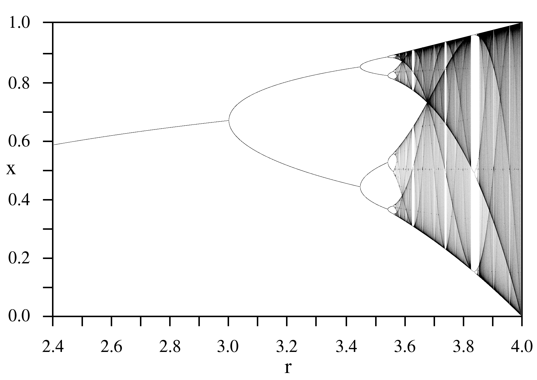
LogisticMap BifurcationDiagram — Bifurcation diagram of a logistic map, displaying chaotic behavior past a threshold

Simple systems can also produce chaos without relying on differential equations. An example is the logistic map, which is a difference equation (recurrence relation) that describes population growth over time.

Even the evolvement of simple discrete systems, such as cellular automata, can heavily depend on initial conditions. Stephen Wolfram has investigated a cellular automaton with this property, termed by him rule 30.

A minimal model for conservative (reversible) chaotic behavior is provided by Arnold's cat map.

Other examples of chaotic systems

Double pendulum
Logistic map
Arnold's cat map
Hénon map
Lorenz model
Smale horseshoe
Dynamical billiards
Chua's circuit
Rössler Map
Economic bubble

Application

Chaos theory is applied in many scientific disciplines: mathematics, biology, computer science, economics, engineering, philosophy, physics, politics, population dynamics, psychology, robotics, etc.[1]

References & Bibliography

This article or section needs to be wikified. Please format this article according to the guidelines laid out at Psychology wiki:Guide to layout. Please remove this template after wikifying.

Li, T. Y. and Yorke, J. A. "Period Three Implies Chaos." Amer. Math. Monthly 82, 985-992, 1975.

Textbooks

Ott, Edward (2002). Chaos in Dynamical Systems, Cambridge University Press New, York. ISBN 0521010845.
Gutzwiller, Martin (1990). Chaos in Classical and Quantum Mechanics, Springer-Verlag New York, LLC. ISBN 0387971734.
Moon, Francis (1990). Chaotic and Fractal Dynamics, Springer-Verlag New York, LLC. ISBN 0471545716.
Tufillaro, Abbott, Reilly (1992). An experimental approach to nonlinear dynamics and chaos, Addison-Wesley New York. ISBN 0201554410.
Gollub, J. P.; Baker, G. L. (1996). Chaotic dynamics, Cambridge University Press. ISBN 0521476852.
Baker, G. L. (1996). Chaos, Scattering and Statistical Mechanics, Cambridge University Press. ISBN 0521395119.
Alligood, K. T. (1997). Chaos: an introduction to dynamical systems, Springer-Verlag New York, LLC. ISBN 0387946772.
Kiel, L. Douglas; Elliott, Euel W. (1997). Chaos Theory in the Social Sciences, Perseus Publishing. ISBN 0472084720.
Strogatz, Steven (2000). Nonlinear Dynamics and Chaos, Perseus Publishing. ISBN 0738204536.
Sprott, Julien Clinton (2003). Chaos and Time-Series Analysis, Oxford University Press. ISBN 0198508409.
Hoover, William Graham (1999,2001). Time Reversibility, Computer Simulation, and Chaos, World Scientific. ISBN 981-02-4073-2.

Semitechnical and popular works

The Beauty of Fractals, by H.-O. Peitgen and P.H. Richter
Chance and Chaos, by David Ruelle
Computers, Pattern, Chaos, and Beauty, by Clifford A. Pickover
Fractals, by Hans Lauwerier
Fractals Everywhere, by Michael Barnsley
Order Out of Chaos, by Ilya Prigogine and Isabelle Stengers
Chaos and Life, by Richard J Bird
Does God Play Dice?, by Ian Stewart
The Science of Fractal Images, by Heinz-Otto Peitgen and Dietmar Saupe, Eds.
Explaining Chaos, by Peter Smith
Chaos: Making a New Science, New York: Penguin, by James Gleick
Complexity, by M. Mitchell Waldrop
Chaos, Fractals and Self-organisation, by Arvind Kumar
Chaotic Evolution and Strange Attractors, by David Ruelle
Sync: The emerging science of spontaneous order, by Steven Strogatz
The Essence of Chaos, by Edward Lorenz
Deep Simplicity, by John Gribbin
The Road To Chaos, by Yoshisuke Ueda
The Chaos Avant-Garde: Memoirs of the Early Days of Chaos Theory, Edited by Ralph H. Abraham and Yoshisuke Ueda

External links

Research Group with Animations in Flash
Nick's Nonlinear Dynamics Archive
Chaos Theory and Education
Chaos Theory: A Brief Introduction
An introduction to Chaos by David M. Harrison, Dept. of Physics. Univ. of Toronto
The Chaos Hypertextbook. An introductory primer on chaos and fractals.
Chaos Theory in the Social Sciences, edited by L Douglas Kiel, Euel W Elliott.
Society for Chaos Theory in Psychology & Life Sciences
Emergence of Chaos at cut-the-knot
Interactive live chaotic pendulum experiment, allows users to interact and sample data from a real working damped driven chaotic pendulum
Nonlinear dynamics: how science comprehends chaos, talk presented by Sunny Auyang, 1998.
New England Complex Systems Institute - Concepts: Chaos

This page uses Creative Commons Licensed content from Wikipedia (view authors).